k-nearest neighbors algorithm

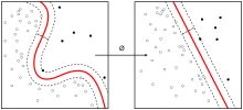
In pattern recognition, the k-nearest neighbors algorithm (k-NN) is a non-parametric method used for classification and regression. In both cases, the input consists of the k closest training examples in the feature space. The output depends on whether k-NN is used for classification or regression:Fig. 1. The dataset.Fig. 2. The 1NN classification map.Fig. 3. The 5NN classification map.Fig. 4. The CNN reduced dataset.Fig. 5. The 1NN classification map based on the CNN extracted prototypes. In pattern recognition, the k-nearest neighbors algorithm (k-NN) is a non-parametric method used for classification and regression. In both cases, the input consists of the k closest training examples in the feature space. The output depends on whether k-NN is used for classification or regression: k-NN is a type of instance-based learning, or lazy learning, where the function is only approximated locally and all computation is deferred until classification. Both for classification and regression, a useful technique can be to assign weights to the contributions of the neighbors, so that the nearer neighbors contribute more to the average than the more distant ones. For example, a common weighting scheme consists in giving each neighbor a weight of 1/d, where d is the distance to the neighbor. The neighbors are taken from a set of objects for which the class (for k-NN classification) or the object property value (for k-NN regression) is known. This can be thought of as the training set for the algorithm, though no explicit training step is required. A peculiarity of the k-NN algorithm is that it is sensitive to the local structure of the data. Suppose we have pairs ( X 1 , Y 1 ) , ( X 2 , Y 2 ) , … , ( X n , Y n ) {displaystyle (X_{1},Y_{1}),(X_{2},Y_{2}),dots ,(X_{n},Y_{n})} taking values in R d × { 1 , 2 } {displaystyle mathbb {R} ^{d} imes {1,2}} , where Y is the class label of X, so that X | Y = r ∼ P r {displaystyle X|Y=rsim P_{r}} for r = 1 , 2 {displaystyle r=1,2} (and probability distributions P r {displaystyle P_{r}} ). Given some norm ‖ ⋅ ‖ {displaystyle |cdot |} on R d {displaystyle mathbb {R} ^{d}} and a point x ∈ R d {displaystyle xin mathbb {R} ^{d}} , let ( X ( 1 ) , Y ( 1 ) ) , … , ( X ( n ) , Y ( n ) ) {displaystyle (X_{(1)},Y_{(1)}),dots ,(X_{(n)},Y_{(n)})} be a reordering of the training data such that ‖ X ( 1 ) − x ‖ ≤ ⋯ ≤ ‖ X ( n ) − x ‖ {displaystyle |X_{(1)}-x|leq dots leq |X_{(n)}-x|} . The training examples are vectors in a multidimensional feature space, each with a class label. The training phase of the algorithm consists only of storing the feature vectors and class labels of the training samples. In the classification phase, k is a user-defined constant, and an unlabeled vector (a query or test point) is classified by assigning the label which is most frequent among the k training samples nearest to that query point. A commonly used distance metric for continuous variables is Euclidean distance. For discrete variables, such as for text classification, another metric can be used, such as the overlap metric (or Hamming distance). In the context of gene expression microarray data, for example, k-NN has been employed with correlation coefficients, such as Pearson and Spearman, as a metric. Often, the classification accuracy of k-NN can be improved significantly if the distance metric is learned with specialized algorithms such as Large Margin Nearest Neighbor or Neighbourhood components analysis.